CPE Performance Analysis Tools User Guide

About the HPE Performance Analysis Tools user guide

The CPE Performance Analysis Tools User Guide provides information about HPE Performance Analysis Tools, which comprises HPE Cray Perftools, HPE Cray Apprentice2, and HPE Cray Reveal. While using this guide, note that:

Because different systems feature a variety of processors, coprocessors, GPU accelerators, and network interconnects, in addition to supporting a variety of compilers, exact results might vary from the examples discussed in this guide. Additionally, not all tools are available on all platforms on which the HPE Cray Programming Environment (CPE) is installed.
This guide is intended for anyone who writes, ports, or optimizes software applications for use on systems running CPE. Users need to be familiar with Linux commands, application development and execution, and general program optimization principles. These tools are best used on an application that is already debugged and capable of running to planned termination.

HPE Performance Analysis Tools

HPE Performance Analysis Tools (Perftools) is a suite of utilities that enable users to capture and analyze performance data generated during program execution, thereby reducing the time to port and tune applications. These tools provide an integrated infrastructure for measurement, analysis, and visualization of computation, communication, I/O, and memory utilization to help users optimize programs for faster execution and more efficient computing resource usage. The data collected and analyzed by these tools help users answer two fundamental developer questions: What is the performance of my program? and How can I make it perform better?

The toolset allows developers to perform profiling, sampling, and tracing experiments on executables, extracting information at the program, function, loop, and line level. Programs written in Fortran, C/C++ (including UPC), Python, MPI, SHMEM, OpenMP, CUDA, HIP, OpenACC, or a combination of these languages and models, are supported. Profiling applications built with the HPE Cray Compiling Environment (CCE), AMD, AOCC, GNU, Intel, Intel OneAPI, or Nvidia HPC SDK compilers are supported. However, not all combinations of programming models are supported, and not all compilers are supported on all platforms. For platform specifics regarding the HPE Cray Programming Environment see Additional Resources.

Performance analysis consists of three basic steps:

Instrument the program to specify what kind of data to collect under what conditions.
Execute the instrumented executable to generate and capture designated data.
Analyze the data.

Available programming interfaces include:

Perftools-lite: Simple interface that produces reports to stdout. Five Perftools-lite submodules exist:
- perftools-lite - Lowest overhead sampling experiment identifies key program bottlenecks.
- perftools-lite-events - Produces a summarized trace; a good tool for detailed MPI statistics, including synchronization overhead.
- perftools-lite-loops - Provides loop work estimates (must be used with CCE).
- perftools-lite-gpu - Focuses on program use of GPU accelerators.
- perftools-lite-hbm - Reports memory traffic information (must be used with CCE and only for Intel processors).
  
  See the perftools-lite(4) man page for details.
Perftools - Advanced interface that provides full-featured data collection and analysis capability, including full traces with timeline displays. Components include:
- pat_build - Utility that instruments programs for performance data collection.
- pat_report - After using pat_build to instrument the program, setting the runtime environment variables and executing the program, use pat_report to generate text reports from the resulting data and export the data to other applications. See the pat_report(1) man page for details.
- CrayPat runtime library - Collects specified performance data during program execution. See the intro_craypat(1) man page for details.
Perftools-preload - Runtime instrumentation version of the performance analysis tools, which eliminates the instrumentation step by pat_build on an executable program. perftools-preload acquires performance data about the program, providing access to nearly all performance analysis features provided by executing a program instrumented with pat_build. See the perftools-preload(4) man page for more details.
- pat_run - An option for programs built with or without perftools-preload. The program is instrumented during runtime, and collected data can be explored further with pat_report and Apprentice2 tools. See the pat_run(1) man page for details.

Experiments available include:

Sampling experiment - A lightweight experiment that interrupts the program at specific intervals to gather data.
Profiling experiment - A tracing experiment that summarizes collected data.
Tracing experiment - A full-trace experiment that provides detailed information.

Also included:

PAPI - The PAPI library, from the Innovative Computing Laboratory at the University of Tennessee in Knoxville, is distributed with HPE Performance Analysis Tools. PAPI allows applications or custom tools to interface with hardware performance counters made available by the processor, network, or accelerator vendor. Perftools components use PAPI internally for CPU, GPU, network, power, and energy performance counter collection for derived metrics, observations, and performance reporting. A simplified user interface, which does not require the source code modification of using PAPI directly, is provided for accessing counters.
Apprentice2 - An interactive X Window System tool for visualizing and manipulating performance analysis data captured during program execution. Mac and Windows clients are also available.
pat_view - Aggregates and presents multiple sampling experiments for program scaling analysis. See the pat_view(1) man page for more information.
Reveal - Extends technology by combining performance statistics, program source code visualization, and CCE compiler optimization feedback to better identify and exploit parallelism, and to pinpoint memory bandwidth sensitivities in an application. Reveal enables navigation through source code to highlighted dependencies or bottlenecks discovered during optimization. Using the program library provided by CCE and collected performance data, users can understand which high-level loops benefit from loop-level optimizations such as exposing vector parallelism. Reveal provides dependency and variable scoping information for those loops and assists users with creating parallel directives. A Mac client is available for Reveal.
pat_info - Generates a quick summary statement of the contents of a CrayPat experiment data directory.
pat_opts - Displays compile and link options used to prepare files for performance instrumentation.

Use performance tools to:

Identify bottlenecks
Find load-balance and synchronization issues
Find communication overhead issues
Identify loops for parallelization
Map memory bandwidth utilization
Optimize vectorization
Collect application energy consumption information
Collect scaling information
Interpret performance data

Overview of HPE Cray Apprentice2

HPE Cray Apprentice2 is a graphical user interface (GUI) tool for visualizing and manipulating performance analysis data captured during program execution. It can display a wide variety of reports and graphs. The number and appearance of the reports when using Apprentice2 is determined by the kind and quantity of data captured during program execution, the type of program being analyzed, the way in which the program is instrumented, and the environment variables in effect at the time of program execution.

Apprentice2 is not integrated with performance tools. Users cannot set up or run performance analysis experiments from within Apprentice2, nor can they launch Apprentice2 from within performance tools. To deploy the tool, use pat_build to instrument the program and capture performance data, then use pat_report to process the raw data (saved in .xf format) and convert it to .ap2 format. Perftools-lite modules, when loaded, automatically carry out these steps and generate .ap2 files. Use Apprentice2 to visualize and explore the resulting .ap2 data files.

You can experiment with the Apprentice2 user interface and left- or right-click on any selected area. Because Apprentice2 does not write any data files, it cannot corrupt, truncate, or otherwise damage the original experiment data. However, under some circumstances, it is possible to use the Apprentice2 text report to overwrite generated MPICH_RANK_ORDER files. If this happens, use pat_report to regenerate the rank order files from the original .ap2 data files. For more information, see MPI Automatic Rank Order Analysis.

Both Windows and Mac clients are available for Apprentice2.

Source code analysis using Reveal

Reveal is an integrated performance analysis and code optimization tool. Reveal extends existing performance measurement, analysis, and visualization technology by combining runtime performance statistics and program source code visualization with CCE compile-time optimization feedback.

Reveal supports source code navigation using whole-program analysis data and program libraries provided by the CCE, coupled with performance data collected during program execution by the performance tools, to understand which high-level serial loops could benefit from improved parallelism. Reveal provides enhanced loopmark listing functionality, dependency information for targeted loops, and assists users optimizing code by providing variable scoping feedback and suggested compiler directives. To begin using Reveal, see HPE Cray Reveal.

A Mac client is available for Reveal.

Available help

The CrayPat man pages, command-line driven help, and FAQ are available only if the perftools-base module is loaded.

The Perftools, Apprentice2, and Reveal commands, options, and environment variables are documented in the following man pages:

app2(1) - Using Apprentice2 for visualizing and manipulating performance analysis data.
grid_order(1) - Optional CrayPat standalone utility that generates MPI rank order placement files (MPI programs only).
intro_craypat(1) - Basic usage and environment variables for Perftools.
pat_build(1) - Instrumenting options and API usage for Perftools.
pat_help(1) - Accessing and navigating pat_help, the command-line driven help system for CrayPat.
pat_info(1) - Querying the Perftools experiment data directory.
pat_opts(1) - Compile and link options for Perftools.
pat_report(1) - Reporting and data-export options.
pat_run(1) - Launch a program to collect performance information.
pat_view(1) - a graphical analysis tool used to view CrayPat data.
reveal(1) - Introduction to the Reveal integrated code analysis and optimization assistant.
perftools-lite(4) - Basic usage information for the Perftools-lite submodules.
perftools-preload(4)- Description of runtime instrumentation of Perftools.
accpc(5) - Optional GPU accelerator performance counters that can be enabled during program execution.
cray_cassini(5) - Network performance counter groups for the HPE Cray Cassini NIC.
cray_pm(5)- Optional Power Management (PM) counters that, when enabled, provide node-level data during program execution (HPE Cray Supercomputing EX systems only).
cray_rapl(5)- Optional Intel Running Average Power Limit (RAPL) counters that, when enabled, provide socket-level data during program execution.
hwpc(5) - Optional CPU performance counters that can be enabled during program execution.
uncore(5) - Optional Intel performance counters that reside off-core and can be enabled during program execution.

See the following man pages for additional information.

intro_mpi(3) - Introduction to the MPI library, including information about using MPICH rank reordering information produced by Perftools; this man page is available only when the cray-mpich module is loaded.
intro_papi(3) - Introduction to the PAPI library, including information about using PAPI to address hardware and network program counters.
papi_counters(5) - Additional information about PAPI utilities.

HPE Cray Perftools help

pat_help is an extensive command-line driven help system that features many examples and answers to many frequently asked questions. To access help, enter:

$ pat_help

The pat_help command accepts options. For example, to jump directly into the FAQ:

$ pat_help FAQ

After the help system is launched, navigation is by single key commands (for example, use “/” to return to the top-level menu), and text menus. It is not necessary to enter entire words to make a selection from a text menu; only the significant letters are required. For example, to select “Building Applications” from the FAQ menu, entering Buil is adequate.

Help system usage is documented further in the pat_help(1) man page.

HPE Cray Apprentice2 help

Apprentice2 offers an integrated help system as well as numerous pop-ups and tool tips that are displayed by hovering the cursor over an area of interest on a chart or graph. You can access the Apprentice2 help system in two ways:

Select Panel Help from the Help drop-down menu; the first page of the help system is displayed.
Right-click on any of the report tabs; the help system opens the report from which the request was made.

HPE Cray Reveal help

Reveal also features an integrated help system with numerous pop-ups and tips that are displayed by hovering the cursor over an area of interest in the source code. You access this integrated help system by clicking Help on the menu bar.

Reference files

If the perftools-base module is loaded, the environment variable CRAYPAT_ROOT is defined. Find useful files in the subdirectories under $CRAYPAT_ROOT/share and $CRAYPAT_ROOT/include.

Subdirectory name	Description
`$CRAYPAT_ROOT/share/config`	Contains build directives (see `pat_build(1)` man page), Automatic Profiling
	Analysis (see Use Automatic Profiling Analysis), report options
	(see `pat_report(1)` man page), `pat_report` pruning, and Perftools-lite
	(see Perftools-lite) configuration files.

`$CRAYPAT_ROOT/share/counters`	Contains hardware-specific performance counter definition files. See
	Monitor Performance Counters.

`$CRAYPAT_ROOT/share/traces`	Contains predefined trace group definitions. See Use Predefined Trace Groups.

`$CRAYPAT_ROOT/include`	Files used with the Perftools API. See CrayPat API for Advanced Users.

`$CRAYPAT_ROOT/share/desktop_installers`	Desktop installer files for:
	- macOS: `Apprentice2Installer-<version_number>.dmg`
	- macOS: `RevealInstaller-<version_number>.dmg`
	- Windows: `Apprentice2Installer-<version_number>.exe`

HPE Cray Perftools

To use the HPE Performance Measurement and Analysis Tools:

Load the programming environment of choice, including CPU or other targeting modules as required:
```
$ module load <PrgEnv>
```
Load the perftools-base module:
```
$ module load perftools-base
```
Load the perftools module for full-feature toolset functionality:
```
$ module load perftools
```
For successful results, load the perftools-base and perftools instrumentation modules before compiling and linking the program to be instrumented, instrumenting the program, executing the instrumented program, or generating a report.

When instrumenting a program, Perftools requires that the object (.o) files created during compilation are present:
```
$ ftn -o <executable> <sourcefile1.o ... sourcefilen.0>
```

See compiler documentation for more information about compiling and linking.

Instrument the Program

Use the pat_build command to instrument the program for performance analysis experiments”

After the perftools-base and perftools instrumentation modules are loaded, and
The program is compiled and linked. For example (in simplest form):
```
$ pat_build <executable> 
```

This procedure produces a copy of the original program, which is saved as <executable>+pat (for example, a.out+pat) and is instrumented for the default experiment. The original executable remains untouched.

The pat_build command supports several options and directives, including an API that enables users to instrument specified regions of code. These options and directives are documented in the pat_build(1) man page. The CrayPat API is discussed in CrayPat API for Advanced Users.

Automatic Profiling Analysis Introduction

The default experiment is Automatic Profiling Analysis, which is an automated process for determining the pat_build options most likely to produce meaningful data from the program. For more information about using Automatic Profiling Analysis, see Use Automatic Profiling Analysis.

MPI Automatic Rank Order Analysis Introduction

Perftools is also capable of:

Performing Automatic Rank Order Analysis on MPI programs and
Generating a suggested rank order list for use with MPI rank placement options.

Use of this feature requires instrumenting the program in pat_build using either the -g mpi or -O apa option. For more information about using MPI Automatic Rank Order Analysis, see MPI Automatic Rank Order Analysis.

`pat_opts`

pat_opts displays compiler and linker options necessary to properly prepare relocatable object files and the resulting executable file for instrumentation by performance utilities. Use pat_opts in situations where CPE modules are not available, or not sufficient, to pass the options needed by Perftools to the build environment. Used properly, these options allow a program to take advantage of the instrumentation analysis provided by the Perftools modules.

If no compiler-designator (for example, cray, gnu) is specified and a PrgEnv module file is loaded, the value of the PE_ENV environment variable is used. Otherwise, pat_opts exits with an error.

The lite-mode operand specifies the name of the Perftools-lite module for which supporting options are generated. Supported values include events, gpu, hbm, lite, loops, and samples. See the perftools-lite(4) man page for more information.

Inserting the options into the respective locations in the compile and link steps facilitates the generation of relocatable object files and an executable file properly formatted for instrumentation processing by the pat_build utility. These options are not mandatory when using pat_run, but they aid data collection when used with runtime instrumentation.

Instrumenting a program using pat_run

Use pat_run to provide some instrumentation to a program that was compiled without the perftools-base module loaded. However, for full Perftools functionality, load the perftools-base and perftools-preload modules and then recompile and relink.

Run the Program and Collect Data

Instrumented programs are executed the same way as the original program; either by using the aprun or srun commands if the site permits interactive sessions or by using system batch commands.

When working on a system, always pay attention to file system mount points. While it may be possible to execute a program on a login node or while mounted on the ufs file system, this action generally does not produce meaningful data. Instead, always opt to run instrumented programs on compute nodes while mounted on a high performance file system, such as the Lustre file system, that supports record locking.

Perftools supports more than 50 optional runtime environment variables that enable users to control instrumented program behavior and data collection during execution. For example, to collect data in detail rather than in aggregate, set the PAT_RT_SUMMARY environment variable to 0 (off) before launching the program.

$ setenv PAT_RT_SUMMARY 0     csh(1)
$ export PAT_RT_SUMMARY=0     bash(1) and sh(1)

Switching off data summarization records detailed data with timestamps and can nearly double the number of reports available in Apprentice2. However, it is typically at the cost of potentially enormous raw data files and significantly increased overhead. Runtime environment variables that control the size of raw data are also available.

The Perftools runtime environment variables are documented in the intro_craypat(1) man page and discussed in CrayPat Runtime Environment.

Analyze the Results

Assuming the instrumented program runs to completion or planned termination, Perftools outputs one or more data files. The exact number, location, and content of the data file(s) varies depending on the nature of the program, the type of experiment for which it was instrumented, and the runtime environment variable settings in effect at the time of program execution.

All initial data files are written to files with an .xf suffix and stored in an experiment data directory generated by the instrumented program. The data directory has the following naming convention:

<my_program>+pat+<PID>-<node>[s|t]

where:

<my_program> = original program name
<PID> = execution process ID number
<node> = execution node number
[s|t] = type of experiment performed, either “s” for sampling or “t” for tracing

Depending on the program executed and the types of data collected, Perftools output consists of either a single .xf data file or multiple .xf data files located in an xf-files directory within the experiment data directory.

Invoke pat_report for the experiment data directory promptly after the completion of program execution in order to write out the runtime results and analysis, and produce the .ap2 file(s). This ensures the mapping of addresses in dynamic libraries to function names uses the same versions of those libraries used when the program was executed.

Initial Analysis Using pat_report

Use pat_report to begin analyzing the captured data. For example (in simplest form):

$ pat_report <my_program>+pat+<PID>-<node>[s|t]

The pat_report command:

Accepts the experiment data directory name as input and processes the .xf file(s) to generate a text report. It also exports the .xf data within the xf-files directory to one or more .ap2 files in an ap2-files directory created within the experiment data directory. The ap2-files directory is a self-contained archive that can later be opened by pat_report or Apprentice2.
- An additional data file named index.ap2 is generated within the experiment data directory.
  
  WARNING: Do not delete the index.ap2 file.
Can be invoked within the experiment data directory by giving ap2-files, xf-files, or index.ap2 as an input argument.
Provides more than 30 predefined report templates as well as numerous user-configurable options, including data export options such as the ability to generate .csv or .html files. These reports and options are discussed in Use pat_report. For more information, see the pat_report(1) man page.

HPE Cray Perftools-lite

Perftools-lite is a simplified version of the HPE Performance Measurement and Analysis Tool set. It provides basic performance analysis information automatically with minimal user interaction. This basic performance analysis information can be foundational to users needing to further explore program behavior using the full Perftools tool set.

Instrumentation module options

The perftools-lite instrumentation modules support five basic experiments:

perftools-lite: A sampling experiment that reports execution time, vector intensity, memory traffic (including stalls), top time-consuming functions and routines, MPI behavior in user functions (if an MPI program), and generates data files.

Perftools-lite limitations: As a special mode of Perftools, Perftools-lite is designed to provide performance data with minimal impact to job wall-clock time. However, execution using a large number of ranks, and/or large number of threads, can greatly increase the post-processing time required for report generation. This issue can be further exacerbated by long-running jobs, application characteristics (such as deep call trees), and other factors. If the post-processing time for the job is excessive with Perftools-lite, set PAT_RT_REPORT_METHOD=0 in the job script. This setting bypasses the Perftools-lite post-processing normally done at job end. The data is written out and can be post-processed using pat_report.
perftools-lite-events: A tracing experiment that generates a profile of the top functions traced, node observations, and possible rank order suggestions.
perftools-lite-gpu: Focuses on application use of GPU accelerators.
perftools-lite-loops: Information on loop trip counts and execution times (for use with Reveal).
perftools-lite-hbm: Identifies data objects that cause the highest load bandwidth from memory (for use with Reveal).

Getting started with HPE Cray Perftools-lite

Perftools-lite automatically instruments a program at compile time when one of the instrumentation modules listed in Instrumentation Module Options is loaded. The perftools-base module must also be loaded.

Note that the instrumented program is saved using the original program name. The executable without instrumentation is saved using the original program name suffixed with +orig.

Load a perftools-lite instrumentation module:

$ module load perftools-base
$ module load <perftools_lite_module>

Compile and link a program:
```
$ make <my_program>
```
Run the executable:
```
$ aprun <a.out>
```

Generated output

At the end of normal program execution, Perftools-lite generates:

A text report to stdout that profiles program behavior, identifies where the program spends its execution time, and offers recommendations for further analysis and possible optimizations.
An experiment data directory containing files for examining the program’s behavior in more detail with Apprentice2, pat_report, or Reveal.
A report file saved to <data-directory>/rpt-files/RUNTIME.rpt containing the same information written to stdout.
For MPI programs, one or more MPICH_RANK_ORDER_FILE files that are saved to the experiment data directory, each containing suggestions for optimizing MPI rank placement in subsequent program runs. The number and types of files produced is determined by the information captured during program execution. The files can include rank reordering suggestions based on sent message data from MPI functions, time spent in user functions, or a hybrid of the two.

Disable HPE Cray Perftools-lite

To disable Perftools-lite during a build, unload the specific perftools-lite instrumentation module. If built with a Perftools-lite module, an executable is instrumented and initiates Perftools functionality at runtime whether or not a Perftools-lite module is still loaded. Relinking with a different Perftools-lite module loaded reinstruments the executable.

Use HPE Cray Perftools-lite

PREREQUISITES

Load the perftools-base module before completing this procedure.

PROCEDURE

Load the desired Perftools-lite instrumentation module:
```
$ module load <perftools_lite_module>
```
Compile and link the program:
```
$ make <my_program>
```
All .o files generated during this step are saved automatically.
Run the program:
```
$ aprun <a.out>
```
Review the resulting reports from the default profiling experiment. To continue with another experiment, delete or rename the <a.out> file. This forces a subsequent make to relink the program for a new experiment.
```
$ rm <a.out>
```
Swap to a different instrumentation module (see Instrumentation Module Options):
```
$ module swap <perftools_lite_module1> <perftools_lite_module2>
```
Rerun make. Because the .o files are saved from the compile step, this merely relinks the program.
```
$ make <my_program>
```
Run the program again:
```
$ aprun <a.out>
```
Review the resulting reports and data files, and determine whether to explore program behavior further using the full Perftools tool set or use one of the MPICH_RANK_ORDER_FILE files to create a customized rank placement. For more information about customized rank placements, see the instructions contained in the MPICH_RANK_ORDER_FILE and the intro_mpi(3) man page.
Identify application bottlenecks by reviewing the profiling reports written to stdout. Use the pat_report utility on the experiment directory produced by a profiling run (for example, <my_program>+<PID>+<node>s) to generate new text reports and additional information without re-running the program.

To disable Perftools-lite during a build, unload the specific perftools-lite instrumentation module. If built using a Perftools-lite instrumentation module, an executable is instrumented and initiates Perftools functionality at runtime even if a Perftools-lite instrumentation module is still loaded. Relinking with a different Perftools-lite instrumentation module that is loaded reinstruments the executable.

Use pat_build

Program instrumentation

The pat_build utility is the instrumenting component of the CrayPat performance analysis tool. After loading the perftools-base and perftools modules and recompiling the program, use the pat_build utility to instrument the program for data capture.

Note that:

Only dynamically-linked executable files are eligible for instrumentation by pat_build.
An application must be free of compilation and runtime errors before instrumentation by pat_build.

CrayPat supports two categories of performance analysis experiments:

Tracing experiments that count some event, such as the number of times a specific system call is executed
Asynchronous (sampling) experiments that capture values at specified time intervals or when a specified counter overflows

The pat_build utility is documented in more detail in the pat_build(1) man page. Access additional information and examples using pat_help, a command-line driven help system, by executing pat_help build.

Basic profiling

The easiest way to use the pat_build command is by accepting the defaults, which generates a copy of the original executable that is instrumented for the default experiment, automatic profiling analysis. A variety of other predefined experiments are available (see Select a Predefined Experiment); however, Automatic Profiling Analysis is usually the best place to start.

Use automatic profiling analysis

The automatic profiling analysis feature lets CrayPat suggest how the program should be instrumented in order to capture the most useful data from the most interesting areas.

Instrument the original program:
```
$ pat_build <my_program>
```
This produces the <my_program>+pat instrumented program.
Run the instrumented program:
```
$ aprun <my_program>+pat
```
This produces the <my_program>+pat+<PID>-<node>s experiment data directory.
Use pat_report to process the experiment data:
```
$ pat_report <my_program>+pat+<PID>-<node>s
```
Performing this step produces:
- A sampling-based text report to stdout,
- One or more .ap2 files, <my_program>+pat+<PID>-<node>s/ap2-files/*, that contain the report data and the associated mapping from addresses to functions and source line numbers, and
- An .apa file, <my_program>+pat+<PID>-<node>s/build-options.apa, that contains the pat_build arguments recommended for further performance analysis.
Reinstrument the program, using the .apa file:
```
$ pat_build -O <my_program>+pat+<PID>-<node>s/build-options.apa
```
It is not necessary to specify the program name, as it is specified in the .apa file. Invoking this command produces the new <my_program>+apa executable, now instrumented for enhanced tracing analysis.
Run the new instrumented program:
```
$ aprun <my_program>+apa
```
The new <my_program>+apa+<PID2>-<node>t experiment data directory, which contains expanded information tracing the most significant functions, is created.
Use pat_report to process the new data file:
```
$ pat_report <my_program>+apa+<PID2>-<node>t
```
This produces the following output:
- A tracing report to stdout
- ap2-files within <my_program>+pat+<PID2>-<node>t containing both the report data and the associated mapping from addresses to functions and source line numbers
- An ap2-files directory within <my_program>+pat+<PID2>-<node>t containing the new data files

If certain conditions are met (for example, job size, data availability), pat_report also attempts to detect a grid topology and evaluate alternative rank orders for opportunities to minimize off-node message traffic, while also trying to balance user time across the cores within a node. These rank-order observations appear on the profile report, and depending on the results, pat_report might also generate one or more MPICH_RANK_ORDER files for use with the MPICH_RANK_REORDER_METHOD environment variable in subsequent application runs.

For more information about MPI rank order analysis, see MPI Automatic Rank Order Analysis. For more information about Automatic Profiling Analysis, see the APA topic in pat_help.

Use Predefined Trace Groups

After Automatic Profiling Analysis, the next-easiest way to instrument the program for tracing is by using the -g option to specify a predefined trace group:

$ pat_build -g <tracegroup> <my_program>

These trace groups instrument the program to trace all function references belonging to the specified group. Only those functions executed by the program at runtime are traced. <tracegroup> is case-insensitive and can be one or more of the values listed in the table. If the exclamation point (!) character appears before <tracegroup>, the functions within the specified trace group are not traced.

See the pat_build(1) manpage for an up-to-date list of trace groups.

Trace Groups:

adios2 - Adaptable I/O System API
aio - Functions that perform Asynchronous I/O
blacs - Basic Linear Algebra Communication Subprograms
blas - Basic Linear Algebra Subprograms
caf - Co-Array Fortran (CCE only)
comex - Communications Runtime for Extreme Scale
cuda - NVIDIA Compute Unified Device Architecture Runtime and Driver API
cuda_math - NVIDIA Compute Unified Device Architecture Math Library API
curl - Multi-protocol File Transfer API
dl - Functions that Perform Dynamic Linking
dmapp - Distributed Memory Application API
dsmml - Distributed Shared Symmetric Memory Management API
fabric - Open Network Communication Services API
ffio - Functions that perform Flexible File I/O (CCE only)
fftw - Fast Fourier Transform Library
ga - Global Arrays API
gmp - GNU Multiple Precision Arithmetic Library
hdf5 - Hierarchical Data Format Library
heap - Dynamic Heap
hip - AMD Heterogeneous-compute Interface for Portability Runtime API
hip_math - AMD Heterogeneous-compute Interface for Portability Math Library API
hsa - AMD Heterogeneous System Architecture API
huge - Linux Huge Pages
io - Functions and System Calls that Perform I/O
lapack - Linear Algebra Package
lustre - Lustre User API
math - POSIX.1 Math Definitions
memory - Memory Management Operations
mpfr - GNU Multiple Precision Floating-Point Library
mpi - MPI
nccl - NVIDIA Collective Communication Library
netcdf - Network Common Data Form
numa - Non-uniform Memory Access API (see numa(3))
oacc - OpenAccelerator API
omp - OpenMP API
opencl - Open Computing Language API
pblas - Parallel Basic Linear Algebra Subroutines
petsc - Portable Extensible Toolkit for Scientific Computation (supported for “real” computations only)
pgas - Parallel Global Address Space
pnetcdf - Parallel Network Common Data Form (C bindings only)
pthreads - POSIX Threads
pthreads_mutex - POSIX Threads Concurrent Process Control
pthreads_spin - POSIX Threads Low-level Synchronization Control
rccl - AMD ROCm Communication Collectives Library
realtime - Scalable LAPACK
rocm_math - AMD Radeon Open Compute Platform Math Library API
shmem - Cray SHMEM
signal - POSIX Signal Handling and Control
spawn - POSIX Real-time Process Creation
stdio - All Library Functions that Accept or Return the FILE* Construct
string - String Operations
syscall - System Calls
sysfs - System Calls that Perform Miscellaneous File Management
sysio - System Calls that Perform I/O
umpire - Heterogeneous Memory Resources Management Library
upc - Unified Parallel C (CCE only)
xpmem - Cross-process Memory Mapping
zmq - High-performance Asynchronous Messaging API

The files that define the predefined trace groups are kept in $CRAYPAT_ROOT/share/traces. To see exactly which functions are being traced in any given group, examine the Trace* files. These files can also be used as templates for creating user-defined tracing files. See Instrument a User-defined List of Functions.

The information available for use in pat_report depends on the way in which a program is instrumented using pat_build. For example, to obtain MPI data in any of the reports produced by pat_report, the program must be instrumented. It is instrumented to collect MPI information. (Use either the -g mpi option or a user-defined tracing option.) For more information, see Predefined Reports.

The pat_run utility also accepts the -g option to indicate trace groups to instrument at runtime.

Trace User defined Functions

Use the pat_build command options to instrument specific functions, to instrument a user-defined list of functions, to block the instrumentation of specific functions, or to create new trace intercept routines.

Enable Tracing and the CrayPat API

Use the -w option to change the default experiment from Automatic Profiling Analysis to tracing, activate any API calls added to the program, and enable tracing for user-defined functions:

$ pat_build -w <my_program>

The -w option has other implications that are discussed in the following sections.

Instrument a Single Function

Use the -T option to instrument a specific function by name:

$ pat_build -T <tracefunc> <my_program>

Note that:

The -T option only applies to user-defined functions; it does not apply to functions contained within a trace group.
If <tracefunc> is a user-defined function, the -w option must also be specified in order to create a trace wrapper for the function; see Use Predefined Trace Groups. If the -w option is not specified, only those functions that have predefined trace intercept routines are traced.
If <tracefunc> contains a slash (/) character, the string is interpreted as a basic regular expression. If more than one regular expression is specified, the union of all regular expressions is taken. All functions that match at least one of the regular expressions are added to the list of functions to trace. One or more regular expression qualifiers can precede the slash (/) character. The exclamation point (!) qualifier means reverse the results of the match, the i qualifier means ignore case when matching, and the x qualifier means use extended regular expressions. For more information about UNIX regular expressions, see the regexec(3) man page.

Prevent Instrumentation of a Function

Use the -T ! option to prevent instrumentation of a specific function:

$ pat_build -T !<tracefunc> <my_program>

If <tracefunc> begins with an exclamation point (!) character, references to <tracefunc> are not traced.

Instrument a User defined List of Functions

Use the -t option to trace a user-defined list of functions:

$ pat_build -t <tracefile> <my_program>

The <tracefunc> is a plain ASCII text file listing the functions to be traced. For an example of a tracefile, see any of the predefined Trace* files in $CRAYPAT_ROOT/share/traces.

To generate trace wrappers for user-defined functions, also include the -w option. If the -w option is not specified, only those functions that have predefined trace intercept routines are traced.

Create New Trace Intercept Routines for User-defined Functions

Use the -u option to create new trace intercept routines for those functions that are defined in the respective source file owned by the user:

$ pat_build -u <my_program>

Use the -T ! option to prevent a specific function from being traced:

$ pat_build -u -T !<function> <my_program>

CrayPat API for Advanced Users

To focus on a certain region within the code:

Reduce sampling or tracing overhead,
Reduce data file size, or
When only a particular region or function is of interest, use the CrayPat API to insert calls into the program source and turn data capture on and off at key points during program execution.

Using the CrayPat API, it is possible to collect data for specific functions. It occurs upon entry into and exit from them, or even from one or more regions within the body of a function.

Use CrayPat API Calls

Procedure

Load the necessary modules:

$ module load perftools-base
$ module load perftools

Include the CrayPat API header file in the source code. Header files for both Fortran and C/C++ are provided in $CRAYPAT_ROOT/include. See Header Files.
Modify the source code by inserting API calls where wanted.
Compile code. Use the pat_build -w option to build the instrumented program. Additional functions can be specified using the -t or -T options. The -u option (see Create New Trace Intercept Routines for User-defined Functions) can be used. It is not recommended, as it forces pat_build to create a function for every user-defined function. This action can inject excessive tracing overhead and obscure the results for the regions.
Run the instrumented program, and use the pat_report command to examine the results.

Header Files

CrayPat API calls are supported in both Fortran and C/C++. The included files are found in $CRAYPAT_ROOT/include.

The pat_api.h C header file must be included in the C source code.

The pat_apif.h and pat_apif77.h Fortran header files provide important declarations and constants and should be included in Fortran source files that reference the CrayPat API. The header file pat_apif.h is used only with compilers that accept Fortran 90 constructs such as new-style declarations and interface blocks. The alternative pat_apif77.h Fortran header file is used with compilers that do not accept such constructs.

CRAYPAT Macro

If the perftools-base module is loaded, it defines a compiler macro called CRAYPAT that can be useful when adding any of the API calls or include statements to the program to make them conditional:

#if defined(CRAYPAT)
<function call>
#endif

This macro can be activated manually by compiling with the -D CRAYPAT argument or otherwise defined by using the #define preprocessor macro.

API Calls

The following are supported API calls. Examples show C syntax; Fortran functions are similar.

All API usage must begin with a PAT_region_begin call and end with a PAT_region_end call, which define region boundaries.

API call	Description
`PAT_region_begin (int <id>, const char *<label>)`	A region consists of a sequence of executable statements
`PAT_region_end (int <id>)`	within a single function and must have a single entry at
	the top and a single exit at the bottom. Regions must be
	either separate or nested; if two regions are not
	disjoint, then one must entirely contain the other. A region
	may contain function calls. These restrictions are similar
	to the restrictions on an OpenMP structured block.

	A summary of activity, including time and performance
	counters (if selected), is produced for each region. The
	argument `<id>` assigns a numerical value to the region and
	must be greater than zero. Each `<id>` must be unique across
	the entire program. The argument `<label`> assigns a
	character string to the region, allowing for easier
	identification of the region in the report.

	These functions return `PAT_API_OK` if the region request is
	valid and `PAT_API_FAIL` if the request is not valid.

	Two runtime environment variables affect region processing:
	`PAT_RT_REGION_CALLSTACK` and `PAT_RT_REGION_MAX`. See the
	`intro_craypat(1)` man page for more information.

`PAT_region_push (const char *<label>)`	When enabled and executed, these functions define the
`PAT_region_pop (const char *<label>)`	beginning and end of a region which is identified by
	the label. The calls from an associated pair are not
	required to appear within the same function, and the same
	label may be used in more than one pair of calls. If an
	execution of one region overlaps in time with an execution
	of another region or a traced function, then the time for
	one must entirely contain the time for the other. For each
	region, a summary of activity, including time and hardware
	performance counters (if selected), is produced. These
	functions return `PAT_API_OK` if the region request was
	valid and `PAT_API_FAIL` if the request was not valid.

`PAT_record (int <state>)`	If called from the main thread, `PAT_record` controls the
	state for all threads on the executing PE. Otherwise, it
	controls the state for the calling thread on the executing
	PE. The function sets the recording `<state>` to one of the
	following values and returns the previous state before the
	call was made.

	Calling `PAT_STATE_ON` or `PAT_STATE_OFF` in the middle of
	a traced function does not affect the resulting time for that
	function. These calls affect only subsequent traced functions
	and any other information those traced functions collect.

	- `PAT_STATE_ON`: If called from the main thread, switches
	recording on for all threads on the executing PE. Otherwise,
	switches recording on for just the calling child thread.
	- `PAT_STATE_OFF`: If called from the main thread, switches
	recording off for all threads on the executing PE. Otherwise,
	switches recording off for just the calling child thread.
	- `PAT_STATE_QUERY`: If called from the main thread, returns
	the state of the main thread on the executing PE. Otherwise,
	returns the state of the calling child thread.

	All other values have no effect on the state.

`PAT_flush_buffer (unsigned long *<nbytes>)`	Writes all the recorded contents in the data buffer to the
	experiment data file for the calling PE and calling thread.
	The number of bytes written to the experiment data file is
	returned in the variable pointed to by `<nbytes>`.

	The function returns `PAT_API_OK` if all buffered data was
	written to the data file successfully; otherwise, it returns
	`PAT_API_FAIL`. After writing the contents, the data buffer
	is empty and begins to refill. See `intro_craypat(1)` to
	control the size of the write buffer.

`PAT_heap_stats`	When enabled and executed in full trace mode, the system
	records dynamic heap information.

`PAT_counters (int <category>, const char`	Returns the names and current count value of counter events
`*<names>,` `unsigned long <values>,`	that are set to count on the hardware `<category>`. The names
`int *<nevents>)`	of these events are returned in the `<names>` array of
	strings, the number of `<names>` is returned in the location
	pointed by to `<nevents>`, and the counts are returned for
	the thread from which the function is called. The values for
	these events are returned in the `<values>` array of
	integers, and the number of values is returned in the
	location pointed by to `<nevents>`.

	The function returns `PAT_API_OK` if all the event names
	returned successfully and `PAT_API_FAIL` if not.

	The values for `<category>` are:

	- `PAT_CTRS_ACCEL`: Performance counters that reside on any
	GPU accelerator
	- `PAT_CTRS_CPU`: Performance counters that reside on the CPU
	- `PAT_CTRS_NETWORK`: Performance counters that reside on the
	network interconnect
	- `PAT_CTRS_PM`: Counters that measure Power Management on a
	compute node
	- `PAT_CTRS_RAPL`: Counters that measure the Intel Running
	Average Power Level on a CPU socket
	- `PAT_CTRS_UNCORE`: Performance counters that reside in
	logical control units off the CPU

	To only get the number of events returned, set `<names>` and
	`<values>` to zero. The event names returned are selected at
	runtime using the `PAT_RT_PERFCTR` environment variable.
	If no event names are specified, the value of `<nevents>` is
	zero.

See the pat_api(1) and pat_build(1) man pages, and the API topic in pat_help for more information about CrayPat API usage.

Using pat_run 

As an alternative to pat_build, pat_run combines many pat_build instrumentation features with the environment variable LD_PRELOAD to execute and profile programs with no application rebuild required. The program collects the performance data and produces the same experiment data directory structure as a program independently instrumented with pat_build.

Although a program instrumented with pat_build has more functionality and greater flexibility in data collection than running a program with pat_run, vpat_run supports many of its instrumentation features. In fact, some programs that pat_build cannot instrument can be instrumented with pat_run. The following table summarizes the major differences between pat_build and pat_run.

`pat_build`	`pat_run`
Functions defined in user-owned files can be individually selected for tracing.	You must use the appropriate compiler option to instrument
	functions in user-owned source files.

Functions belonging to a trace group can be individually selected for
tracing.	All functions in a trace group are traced; selecting an individual
	one selects all functions.

Some lite-mode trace functions are available in user-owned source files.	Functions in user-owned source files are only traced in lite mode
	when instrumented using compiler options.

Python experiments are not supported.	Support for Python experiments is currently in beta stage. See
	the discussion in “Python Experiments (BETA)” in the pat_run
	man page.

A workload manager command is required to use pat_run. If the launching command is missing or invalid, pat_run fails or the program does not execute correctly. See the pat_run(1) man page for details. Additionally, see the aprun(1), mpiexec(1), and srun(1) man pages for information on WLM-compatible launch commands.

To maximize access to runtime performance data collection and recording, load the perftools-preload and perftools-base modules before compiling and linking a program. Programs that are not linked with module perftools or perftools-lite can also be executed using the pat_run utility; however, these programs do not have full access to the instrumentation features. Use the -z option to pass user-collectible parameters to allow pat_run to take full advantage of instrumentation features. See the perftools-lite(4), perftools-preload(4), and pat-run(1) man pages for complete details.

HPE Cray CrayPat runtime environment

Instrumented programs reference several HPE Cray CrayPat runtime environment variables that affect data collection and storage. Detailed descriptions of all runtime environment variables are provided in the intro_craypat(1) man page. You can access additional information using pat_help, a command-line driven help system, by executing pat_help environment.

This section provides a summary of the runtime environment variables and highlights some of those more commonly used.

Control runtime summarization

Environment variable: PAT_RT_SUMMARY

Runtime summarization is enabled by default. When enabled, data is captured in detail but automatically aggregated and summarized before being recorded. This process greatly reduces the size of the resulting experiment data files but at the cost temporal activity and fine-grain detail. Specifically, when running tracing experiments, the formal parameter values and function return values are not saved.

To study data in detail, and particularly to use Apprentice2 to generate charts and graphs, disable runtime summarization by setting PAT_RT_SUMMARY to 0. Doing so can more than double the number of reports available in Apprentice2.

Select a predefined experiment

Environment variable: PAT_RT_EXPERIMENT

By default, pat_build instruments programs for automatic profiling analysis. However, if a program is instrumented for a sampling experiment by using the pat_build -S option, or for tracing by using the pat_build -w, -u, -T, -t, or -g options, then the PAT_RT_EXPERIMENT environment variable can be used to further specify the type of experiment to perform.

Valid experiment types include:

samp_pc_time

The default sampling experiment samples the program counters at regular intervals and records the total program time and the absolute and relative times each program counter is recorded. The default sampling interval is 10,000 microseconds by POSIX timer monotonic wall-clock time, but this can be changed using the PAT_RT_SAMPLING_INTERVAL_TIMER runtime environment variable.
samp_pc_ovfl

This experiment samples the program counters at the overflow of a specified hardware performance counter. The counter and overflow value are specified using the PAT_RT_PERFCTR environment variable.
samp_cs_time

This experiment is similar to the samp_pc_time experiment, but it samples the call stack at the specified interval and returns the total program time and the absolute and relative times each call stack counter is recorded.
samp_cs_ovfl

This experiment is similar to the samp_pc_ovfl experiment but samples the call stack.
trace

Tracing experiments trace the functions that are specified using the pat_build -g, -u, -t, -T, -O, or -w options and record entry into and exit from the specified functions. Only true function calls can be traced; function calls that are inlined by the compiler or that have local scope in a compilation unit cannot be traced. The behavior of tracing experiments is also affected by the PAT_RT_TRACE_DEPTH environment variable.

If a program is instrumented for tracing using PAT_RT_EXPERIMENT to specify a sampling experiment, trace-enhanced sampling is performed.

Trace-enhanced sampling

Environment variable: PAT_RT_SAMPLING_MODE

If pat_build is used to instrument a program for a tracing experiment and then PAT_RT_EXPERIMENT is used to specify a sampling experiment, trace-enhanced sampling is enabled and affects both user-defined functions and predefined function groups. Values can be 0, ignore, 1, raw, 3, or bubble. The default is 0.

Improve tracebacks

In normal operation, HPE Cray CrayPat only writes data files when the buffer is full or the program reaches the end of planned execution. If the program aborts during execution and produces a core dump, performance analysis data is normally lost or incomplete.

If this happens, consider setting PAT_RT_SETUP_SIGNAL_HANDLERS to 0 in order to bypass the CrayPat runtime library and capture the signals the program receives. This results in an incomplete experiment file but a more accurate traceback, which might make it easier to determine why the program aborts.

Alternatively, consider setting PAT_RT_WRITE_BUFFER_SIZE to a value smaller than the default value of 8MB, or using the PAT_flush_buffer API call to force HPE Cray CrayPat to write data. Both cause CrayPat to write data more often, resulting in a more-complete experiment data file.

Measure MPI load imbalance

Environment variable: PAT_RT_MPI_SYNC

In MPI programs, time spent waiting at a barrier before entering a collective can be a significant indication of load imbalance. The PAT_RT_MPI_SYNC environment variable, if set, causes the trace wrapper for each collective subroutine to measure the time spent waiting at the barrier call before entering the collective. This time is reported by pat_report in the function group MPI_SYNC, which is separate from the MPI function group, which shows the time actually spent in the collective.

This environment variable affects tracing experiments only and is set on by default.

Monitor performance counters

Environment variable: PAT_RT_PERFCTR

Use this environment variable to specify CPU, network, accelerator, and power management events to be monitored while performing tracing experiments.

Counter events are specified in a comma-separated list. Event names and groups from all components can be mixed as needed; the tool parses the list and determines which event names or group numbers apply to which components. Use the papi_avail or papi_native_avail commands to list the names of the individual events on the system.

You must run papi_avail or papi_native_avail on compute nodes, not on login nodes or esLogin command lines, to get useful information.

Hardware counters

Alternatively, predefined counter group numbers can be used in addition to, or in place of, individual event names to specify one or more predefined performance counter groups. For complete lists of currently supported hardware counter events organized by processor family, execute pat_help counters.

Accelerator counters

Alternatively, an <acgrp> value can be used in place of the list of event names to specify a predefined performance counter accelerator group. The valid <acgrp> names are listed on the system in $CRAYPAT_ROOT/share/counters/CounterGroups.<accelerator>, where <accelerator> is the GPU accelerator used on the system. They are also available in the accpc(5) man page.

If the <acgrp> value specified is invalid or not defined, <acgrp> is treated as a counter event name. This can cause instrumented code to generate “invalid ACC performance counter event name” error messages or possibly abort during execution. Always verify that the <acgrp> values specified are supported on the type of GPU accelerators being used.

Accelerated applications cannot be compiled with -h profile_generate or -finstrument_loop; therefore, GPU accelerator performance statistics and loop profile information cannot be collected simultaneously.

Power management counters

HPE Cray Supercomputing EX systems support two types of power management counters. The PAPI RAPL component provides socket-level access to Intel Running Average Power Limit (RAPL) counters, while the similar PAPI Power Management (PM) counters provide compute node-level access to additional power management counters. Together, these counters enable users to monitor and report energy usage during program execution.

CrayPat supports experiments that make use of both sets of counters. These counters are accessed through use of the PAT_RT_PERFCTR set of runtime environment variables. When RAPL counters are specified, one core per socket is tasked with collecting and recording the specified events. When PM counters are specified, one core per compute node is tasked with collecting and recording the specified events. The resulting metrics appear in text reports.

To list the available events, use the papi_native_avail command on a compute node and filter for the desired PAPI components. For example:

$ aprun papi_native_avail -i cray_rapl
$ aprun papi_native_avail -i cray_pm

For more information about the RAPL and PM counters, see the cray_rapl(5) and cray_pm(5) man pages.

Use pat_report

Generate text reports

The pat_report command is the text reporting component of the HPE Performance Analysis Tools suite. After using the pat_build command to instrument the program, set the runtime environment variables as desired, and then execute the program. Use the pat_report command to generate text reports from the resulting data and export the data for use in other applications.

The pat_report command is documented in detail in the pat_report(1) man page. You can access additional information using pat_help, a command-line driven help system, by executing pat_help report.

Experiment data directories and files

The data files CrayPat generates vary depending on the type of program being analyzed, the type of experiment for which the program was instrumented, and the runtime environment variables in effect at the time the program was executed. In general, the successful execution of an instrumented program produces one or more .xf files that contain the data captured during program execution.

Unless specified otherwise using runtime environment variables, these files are stored in an experiment data directory with the following naming convention:

<a.out>+pat+<PID>-<node>[s|t]

Where:

<a.out> = name of instrumented program
<PID> = process ID assigned to rank 0 of the instrumented program at runtime
<node> = physical node ID upon which the rank zero process was executed
[s|t] = type of experiment performed, either “s” for sampling or “t” for tracing

The experiment data directory initially contains an xf-files directory that contains the individual .xf files.

Use the pat_report command to process the information in experiment data directory files. Upon execution, pat_report automatically generates an ap2-files directory (containing one or more .ap2 files) and an index.ap2 file. The populated experiment data directory can then be specified as input to Apprentice2 or to pat_report for generation of further reports.

If the executable was instrumented with the pat_build -O apa option, running pat_report on the experiment data directory file(s) also produces a build-options.apa file, which is the file used by Automatic Profiling Analysis. See Use Automatic Profiling Analysis.

Generate Reports

To generate a report, use pat_report <data_directory> to process the experiment data directory containing .xf files.

$ pat_report <a.out>+pat+<PID>-<node>t

The complete syntax of the pat_report command is documented in the pat_report(1) man page.

Running pat_report automatically generates an ap2-files directory within the experiment data directory that can be used later by the pat_report command or by Apprentice2. Also, if the executable was instrumented with the pat_build -O apa option, running pat_report on the experiment data directory file(s) produces a build-options.apa or <data_directory>/build-options.apa file, which is the file used by Automatic Profiling Analysis. See Use Automatic Profiling Analysis.

The pat_report command is a powerful report generator with a wide range of user-configurable options. However, the reports that can be generated are first and foremost dependent on the kind and quantity of data captured during program execution. For example, if a report does not seem to show the level of detail being sought when viewed in Apprentice2, consider rerunning the program with different pat_build options, or different or additional runtime environment variable values. Note that setting PAT_RT_SUMMARY to zero (disabled) enables Time Line panels in Apprentice2 but does not affect the reports available from pat_report.

Predefined Reports

Use pat_report with no inputs for the default report, or use a -O option to specify a predefined report. For example, enter this command to see a top-down view of the calltree.

$ pat_report -O calltree <data_directory>

In many cases, a dependency exists between the way in which a program is instrumented in pat_build and the data subsequently available for use by pat_report. For example, instrument the program using the pat_build -g heap option (or one of the equivalent user-defined pat_build options) to acquire useful data on the pat_report -O heap report. Alternatively, use the pat_build -g mpi option (or one of the equivalent user-defined pat_build options) to acquire useful data on the pat_report -O mpi_callers report.

Use pat_report -O -h to list the predefined reports currently available, including:

accelerator - Shows calltree of accelerator performance data sorted by host time.
accpc - Shows accelerator performance counters.
acc_fu - Shows accelerator performance data sorted by host time.
acc_time_fu - Shows accelerator performance data sorted by accelerator time.
acc_time - Shows calltree of accelerator performance data sorted by accelerator time.
acc_show_by_ct - (Deferred implementation) Shows accelerator performance data sorted alphabetically.
affinity - Shows affinity bitmask for each node. Uses -s pe=ALL and -s th=ALL to see affinity for each process and thread, and uses -s filter_input=<expression> to limit the number of PEs shown.
profile - Shows data by function name only.
callers (or ca) - Shows function callers (bottom-up view).
calltree (or ct) - Shows calltree (top-down view).
ca+src - Shows line numbers in callers.
ct+src - Shows line numbers in calltree.
heap - Implies heap_program, heap_hiwater, and heap_leaks. To show heap_hiwater and heap_leaks information, instrumented programs must be built using the pat_build -g heap option.
heap_program - Compares heap usage at the start and end of the program; shows heap space used and free at the start as well as unfreed space and fragmentation at the end.
heap_hiwater - If the pat_build -g heap option was used to instrument the program, this report option shows the:
- Heap usage “high water” mark,
- Total number of allocations and frees, and
- Number and total size of objects allocated but not freed between the start and end of the program.
heap_leaks - If the pat_build -g heap option was used to instrument the program, this report option shows the largest unfreed objects by call site of allocation and PE number.
himem - Memory high water mark by Numa Node. For nodes with multiple sockets or nodes with Intel KNL processors, the default report typically includes a table showing high water usage by numa node. The table is not shown if all memory was mapped to numa node 0, but it can be explicitly requested with pat_report -O himem.
kern_stats - Shows kernel-level statistics, including the:
- average kernel grid size,
- average block size, and
- average amount of shared memory dynamically allocated for the kernel.
load_balance - Implies load_balance_program, load_balance_group, and load_balance_function. Shows PEs with maximum, minimum, and median times.
load_balance_function - Shows the imb_time (difference between maximum and average time across PEs) in seconds and the imb_time% (imb_time/max_time * NumPEs/(NumPEs - 1)) for the whole program, groups, or functions. For example, an imbalance of 100% for a function means that only one PE spent time in that function.
load_balance_cm - If the pat_build -g mpi option was used to instrument the program, this report option shows the load balance by group with collective-message statistics.
load_balance_sm - If the pat_build -g mpi option was used to instrument the program, this report option shows the load balance by group with sent-message statistics.
load_imbalance_thread - Shows the active time (average over PEs) for each thread number.
loop_nest - Provides a nested view of Loop Inclusive Time. If the -h profile_generate compiler option is used when compiling and linking the program, then the associated table is included in a default report. Other loop reporting options enabled by the -h profile_generate compiler option include:
- loop_callers - Loop Stats by Function and Caller.
- loop_callers+src - Loop Stats by Function and Callsites.
- loop_calltree - Function and Loop Calltree View.
- loop_calltree+src - Function and Loop Calltree with Line Numbers.
- loop_times - Inclusive and Exclusive Time in Loops.
- profile_loops - Profile by Group and Function with Loops.
mpi_callers - Shows MPI sent- and collective-message statistics.
mpi_sm_callers - Shows MPI sent-message statistics.
mpi_coll_callers - Shows MPI collective-message statistics.
mpi_dest_bytes - Shows MPI bin statistics as total bytes.
mpi_dest_counts - Shows MPI bin statistics as counts of messages.
mpi_sm_rank_order - If the pat_build -g mpi option was used to instrument the program, this report option calculates a suggested rank order, based on MPI grid detection and MPI point-to-point message optimization. It uses sent-message data from tracing MPI functions to generate suggested MPI rank order information.
mpi_rank_order - If the pat_build -g mpi option was used to instrument the program, this report option calculate a rank order to balance a shared resource, such as USER time over all nodes. It uses time in user functions, or alternatively, any other metric specified by using the -s mro_metric options to generate suggested MPI rank order information.
mpi_hy_rank_order - If the pat_build -g mpi option was used to instrument the program, this report option calculates a rank order, based on a hybrid combination of mpi_sm_rank_order and mpi_rank_order.
nids - Shows PE to NID mapping.
nwpc - Program network counter activity.
profile_nwpc - NWPC data by Function Group and Function. This table is shown by default if NWPC counters are present in the .ap2 file.
profile_pe.th - Shows the imbalance over the set of all threads in the program.
profile_pe_th - Shows the imbalance over PEs of maximum thread times.
profile_th_pe - For each thread, shows the imbalance over PEs.
program_time - Shows which PEs took the maximum, median, and minimum time for the whole program.
read_stats, write_stats - If the pat_build -g io option was used to instrument the program, these options show the I/O statistics by filename and by PE, with maximum, median, and minimum I/O times.
samp_profile+src - Shows sampled data by line number with each function.
thread_times - For each thread number, shows the average of all PE times and the PEs with the minimum, maximum, and median times.

By default, all reports show either no individual PE values or only the PEs having the maximum, median, and minimum values. To show the data for all PEs, append the suffix _all to any of the predefined report options. For example, the option load_balance_all shows the load balance statistics for all PEs involved in program execution. Use this option with caution, as it can yield lengthy reports.

User-defined Reports 

In addition to the -O predefined report options, the pat_report command supports a wide variety of user-configurable options that enable users to create and generate customized reports.

To create customized reports, pay particular attention to the -s, -d, and -b options.

-s

These options define the presentation and appearance of the report. Options range from layout and labels, to formatting details, and setting thresholds that determine whether some data is considered significant enough to be worth displaying.
-d

These options determine which data appears on the report. The range of data items included also depends on how the program is instrumented. It can also include counters, traces, time calculations, mflop counts, heap, I/O, and MPI data. These options enable users to determine how the displayed values are calculated.
-b

These options determine how data is aggregated and labeled in the report summary.

See the pat_report man page for detailed information on these report options. Find information and examples using pat_help, a command-line driven help system, by executing pat_help report. Use pat_report -s -h or pat_report -b -h to see a combined list of items that can be specified with the -b or d options.

Export Data

When using the pat_report command to view the xf-files data within an experiment data directory, pat_report automatically generates an ap2-files directory that can be used later by pat_report or Apprentice2.

The pat_report -f html option generates reports in html-format files that can be read with any modern web browser. If invoked, this option creates a directory named html-files within the experiment data directory, which contains all generated data files. The default name of the primary report file is pat_report.html. This file name can be changed using the -o option.

To export the rows of a table as comma-separated values, use the option -O export in conjunction with another -O option (for example, pat_report -O mpi_p2p_bytes,export ...). The export option consists of a list of specific formatting options that were tuned for use with mpi_p2p_bytes. View and modify selected options by redirecting the output from pat_report -O export -h to a file (for example, my_export). That file can be edited as needed and used with -O my_export. You can also override individual options on the pat_report command line. For example, to incorporate tab separators instead of commas, use pat_report -O mpi_p2p_bytes,export -s csv_sep=TAB ...

`pat_report` Environment Variables

The pat_report environment variables affect the way in which data is handled during report generation.

PAT_AP2_FILE_MAX

Changes the default limit of 256 on the number of .ap2 files created in lite mode. If the limit is less than the number of .xf files, then one or more .ap2 files contain data from more than one .xf file. The base name of an .ap2 file becomes the base name of the first of those .xf files. PAT_AP2_FILE_MAX can be set to zero or a negative value to disable the limit so that each .ap2 file contains data from only one .xf file.
PAT_AP2_KEEP_ADDRS

Set to 1 to disable compression of sampled addresses. The default behavior, when processing data from .xf files to .ap2 files, is to map all addresses that share the same source file number to a single representative address. This setting can significantly reduce the size of the .ap2 files, reducing the time required to generate reports.
PAT_AP2_PRAGMA

Set to a semi-colon-separated list of SQLite pragmas to be supplied to the SQLite library before reading or writing .ap2 files. The default list is:
```
jounal_mode=OFF
synchronous=OFF
locking_mode=EXCLUSIVE
cache_size=4000
```
PAT_AP2_SQLITE_VFS

Set to unix-none to inhibit file locking. This setting becomes the default for xf_ap2 on Macintosh and Linux systems. Set to DEFAULT to use the SQLite3 library default. Other choices are documented at the SQLite webpage.
PAT_REPORT_HELPER_START_FUNCTIONS

Adds to, or redefines, the list of start functions used by some programming models for helper threads that provide support for the model, but does not directly execute code from an application. The value of this variable should be a comma-separated list of function names. If the value begins with a comma, then functions are added to the default list. Otherwise, they replace the default list. The default list is:
```
__kmp_launch_monitor
cudbgGetAPIVersion
cuptiActivityDisable
_dmappi_error_handler
_dmappi_queue_handler
_dmappi_sr_handler
```
PAT_REPORT_IGNORE_VERSION, PAT_REPORT_IGNORE_CHECKSUM

If set, turns off checking that the version of CrayPat being used to generate the report is the same version, or has the same library checksum, as the version that was used to build the instrumented program.
PAT_REPORT_OPTIONS, PAT_REPORT_POST_OPTIONS

If the -z option is specified on the command line, these environment variables are ignored. Otherwise:
- If set, the options in these environment variables are evaluated before, or after, any options on the command line.
- If not set, the values of these variables recorded in the experiment data file are used, if present.
The first variable provides a convenient means to control the processing and reporting of data during runtime, by means of the pat_report -Q option.
PAT_REPORT_PRUNE_NAME

Prune (remove) functions by name from a report. If not set or set to an empty string, no pruning is done. Set this variable to a comma-delimited list (__pat_, __wrap_, and so forth) to supersede the default list, or begin this list with a comma (,) to append this list to the default list. A name matches if it has a list item as a prefix.
PAT_REPORT_PRUNE_SRC

If not set, the behavior is the same as if set to /lib.

If set to the empty string, all callers are shown.

If set to a non-empty string or to a comma-delimited list of strings, a sequence of callers with source paths containing a string from the list are pruned to leave only the top caller.
PAT_REPORT_PRUNE_NON_USER

If set to 0 (zero), disables the default behavior of pruning based on ownership (by user invoking pat_report) of source files containing the definition of a function.
PAT_REPORT_PYTHONHOME

Specifies the pathname of CPython libraries for Python Experiments. If unset, the pathname is ordered as t* $CRAY_PYTHON_PREFIX if set (for example, by the cray-python module) * $PYTHONHOME if set. Otherwise, pathname is assumed to be /usr/lib/libpython or /usr/lib64/libpython. An improper value leads to missing Python information from reports, Python interpreter frames or details being exposed on Python Experiments.
PAT_REPORT_VERBOSE

If set, produces more feedback about the parsing of the .xf file and includes, in the report, the values of all environment variables that were set at the time of program execution.

See the “Environment Variables” section in pat_report man page for more information about pat_report or related variables.

Automatic Profiling Analysis

Assuming the executable was instrumented using the pat_build -O apa option (default behavior), running pat_report on the experiment data directory also produces a build-options.apa or <data_directory>/build-options.apa file containing the recommended parameters for reinstrumenting the program for more detailed performance analysis. The file is located within the experiment data directory. For more information about Automatic Profiling Analysis, see Use Automatic Profiling Analysis.

MPI Automatic Rank Order Analysis

By default, MPI program ranks are placed on compute node cores sequentially, in SMP style, as described in the intro_mpi(3) man page. Use the MPICH_RANK_REORDER_METHOD environment variable to override this default placement, and in some cases, achieve significant improvements in performance by placing ranks on cores to optimize use of shared resources such as memory or network bandwidth.

The HPE Cray Performance Analysis Tools suite provides several ways to help optimize MPI rank ordering. If program communication patterns are understood well enough to specify an optimized rank order without further assistance, the grid_order utility can be used to generate a rank order list to use as input to the MPICH_RANK_REORDER_METHOD environment variable. For more information, see the grid_order(1) man page.

Alternatively, follow these steps to use CrayPat to perform automatic rank order analysis and generate recommended rank-order placement information.

Use Automatic Rank Order Analysis

Instrument the program using either the pat_build -g mpi or -O apa option.
Execute the program.
Use the pat_report command to generate a report from the resulting experiment data directory.

If certain conditions are met (job size, data availability, and so forth), pat_report attempts to detect a grid topology and evaluate alternative rank orders for opportunities to minimize off-node message traffic while also trying to balance user time across the cores within a node. These rank-order observations appear on the resulting profile report, and depending on the results, pat_report may also automatically generate one or more MPICH_RANK_ORDER files within the experiment data directory for use with the MPICH_RANK_REORDER_METHOD environment variable in subsequent application runs.

Force Rank Order Analysis

Use one of these options to force pat_report to generate an MPICH_RANK_ORDER file.

-O mpi_sm_rank_order
-O mpi_rank_order
-O mpi_hy_rank_order

`-O mpi_sm_rank_order`

(Requires that pat_report was invoked with either the -g mpi or -O apa option.) The -O mpi_sm_rank_order option displays a rank-order table based on MPI sent-message data (message sizes or counts, and rank-distances). pat_report attempts to detect a grid topology and evaluate alternative rank orders that minimize off-node message traffic. If successful, a MPICH_RANK_ORDER.Grid file that can be used to dictate the rank order of a subsequent job is generated. Instructions for doing so are included in the file.

The grid detection algorithm used in the sent-message rank-order report looks for patterns in (at most) three dimensions. Also, note that while use of an alternative rank order may improve performance for MPI message delivery, the effect on the performance of the application as a whole is unpredictable.

A number of related -s options are available to tune the mpi_sm_rank_order report. These include:

mro_sm_metric=Dm|Dc

Used with the -O mpi_sm_rank_order option. If set to Dm, the metric is the sum of P2P message bytes sent and received. If set to Dc, the metric is the sum of P2P message counts sent and received.

Default: Dm
mro_mpi_pct=<value>

Specifies the minimum percentage of total time that MPI routines must consume before pat_report suggests an alternative rank order.

Default: 10 (percent)
rank_cell_dim=m1xm2x...

Specifies a set of cell dimensions to use for rank-order calculations. For example, -s rank_cell_dim=2x3.
rank_grid_dim=m1Xm2X...

Specifies a set of grid dimensions to use for rank-order calculations. For example, -s rank_grid_dim=8x5x3.

`-O mpi_rank_order`

The -O mpi_rank_order option generates an alternate rank order based on a resource metric that can be compared across all PEs and balanced across all nodes. The default metric is USER Time, but other HWPC or derived metrics can be specified. If successful, this option generates a MPICH_RANK_ORDER.USER_Time file.

The following related -s options are available to tune the mpi_rank_order report. These include:

mro_metric=ti|...

Any metric can be specified, but memory traffic hardware performance counter events are recommended.

Default: ti
mro_group=USER|MPI|...

If specified, the metric is computed only for functions in the specified group.

Default: USER

`-O mpi_hy_rank_order`

The -O mpi_hy_rank_order option generates a hybrid rank order from the MPI sent-message and shared-resource metric algorithms in an attempt to gain improvements from both. This option is done only for experiments that contain MPI sent-message statistics and whose jobs ran with at least 24 PEs per node. If successful, this option generates a MPICH_RANK_ORDER.USER_Time_hybrid file.

This option supports the same -s options as both -O mpi_sm_rank_order and -O mpi_rank_order.

Observations and Suggestions

The following is an example showing the rank-order observations generated from default pat_report processing on data from a 2045 PE job running on 32 PEs/node. Additional explanations are found in lines beginning with the + character.

================  Observations and suggestions  ========================

MPI Grid Detection:

    There appears to be point-to-point MPI communication in a 35 X 60
+ ---------------------------------------------------------------------
+ This is the grid that pat_report identified by studying MPI message
+ traffic.  Users can change it via the -s rank_grid_dim option.
+ ---------------------------------------------------------------------

    grid pattern. The 20.3% of the total execution time spent in MPI
+ ---------------------------------------------------------------------
+ This MPI-based rank order is calculated only if this application
+ shows that significant (>10%) time is spent doing MPI-related work.
+ ---------------------------------------------------------------------

    functions might be reduced with a rank order that maximizes
    communication between ranks on the same node. The effect of several
    rank orders is estimated below.

    A file named MPICH_RANK_ORDER.Grid was generated along with this
    report and contains usage instructions and the Custom rank order
    from the following table.
+ ---------------------------------------------------------------------
+ Note that the instructions for using each MPICH_RANK_ORDER file are
+ included within that file.
+ ---------------------------------------------------------------------

         Rank    On-Node     On-Node   MPICH_RANK_REORDER_METHOD 
        Order   Bytes/PE   Bytes/PE%   
                            of Total   
                            Bytes/PE   

        Custom  4.050e+09      34.77%  3
           SMP  2.847e+09      24.45%  1
          Fold  1.025e+08       0.88%  2
    RoundRobin  6.098e+01       0.00%  0
+ ---------------------------------------------------------------------
+ This shows that the Custom rank order was able to arrange the ranks
+ such that 34% of the total MPI message bytes sent per PE stayed within
+ each local compute node (the higher the percentage the better).  In
+ this case, the Custom order was a little better than the default SMP
+ order.
+ ---------------------------------------------------------------------


Metric-Based Rank Order:  

    When the use of a shared resource like memory bandwidth is unbalanced
    across nodes, total execution time may be reduced with a rank order
    that improves the balance.  The metric used here for resource usage
    is: USER Time
+ ---------------------------------------------------------------------
+ USER Time is the default, but can be changed via the -s mro_metric
+ option.
+ ---------------------------------------------------------------------

    For each node, the metric values for the ranks on that node are
    summed.  The maximum and average value of those sums are shown below
    for both the current rank order and a custom rank order that seeks
    to reduce the maximum value.

    A file named MPICH_RANK_ORDER.USER_Time was generated
    along with this report and contains usage instructions and the
    Custom rank order from the following table.

      Rank     Node  Reduction    Maximum   Average 
     Order   Metric     in Max      Value   Value 
               Imb.      Value              

    Current    8.95%             6.971e+04  6.347e+04
     Custom    0.37%     8.615%  6.370e+04  6.347e+04
+ ---------------------------------------------------------------------
+ The Node Metric Imbalance column indicates the difference between the
+ maximum and average metric values over the set of compute nodes.  A
+ lower imbalance value is better, as the maximum value is brought down 
+ closer to the average.
+ ---------------------------------------------------------------------


Hybrid Metric-Based Rank Order:  

    A hybrid rank order has been calculated that attempts to take both
    the MPI communication and USER Time resources into account.
    The table below shows the metric-based calculations along with the
    final on-node bytes/PE value.  A MPICH_RANK_ORDER.USER_Time_hybrid
    file was generated along with this report and contains usage
    instructions for this custom rank order.

      Rank     Node  Reduction    Maximum    Average   On-Node 
     Order   Metric     in Max      Value      Value   Bytes/PE% 
               Imb.      Value                         of Total 
                                                       Bytes/PE 

    Current    8.95%             6.971e+04  6.347e+04  23.82%
     Custom    2.70%      6.43%  6.523e+04  6.347e+04  30.28%
+ ---------------------------------------------------------------------
+ Typically, the hybrid node imbalance and the on-node bytes/PE values 
+ are not quite as good as the best values in the MPI grid-based and 
+ metric-based tables, but the goal is to get them as close as possible
+ while gaining benefits from both methodologies.
+ ---------------------------------------------------------------------

Use HPE Cray Apprentice2

HPE Cray Apprentice2 is an interactive X Window System tool for visualizing and manipulating performance analysis data captured during program execution.

The number and appearance of the reports in HPE Cray Apprentice2 is determined by the kind and quantity of data captured during program execution. For example, setting the PAT_RT_SUMMARY environment variable to 0 (zero) before executing the instrumented program nearly doubles the number of reports available when analyzing the resulting data in Apprentice2. However, it does so at the cost of much larger data files.

In addition to native Apprentice2, desktop versions exist for both Mac and Windows installers. Currently, a Linux version is not available. Installers are found at $CRAYPAT_ROOT/share/desktop_installers.

Copy experiment directories to the local machine or use Open Remote under the File menu. Use Add Comparison File or Add Remote Comparison File for compare functions.

Launch Apprentice2

Load the perftools-base module:
```
$ module load perftools-base
```
Launch Apprentice2 with or without a file or directory name to open on launch:
```
$ app2 [<data_directory>]
```

Apprentice2 requires a workstation configured to host X Window System sessions. If the app2 command returns “cannot open display”, see the system administrator for information about configuring X Window System hosting.

The app2 command supports two options: --cg and --compare. The --cg option launches Apprentice2 with the call graph as the initial panel. The --compare option requires two data sets for a side-by-side comparison, both data sets must have the same experiment and summary types.

For more information about the app2 command, see the app2(1) man page.

Open Data Files

If a valid data file or directory is specified with the app2 command, the file or directory opens, and the data is read in and displayed. Otherwise, a default Apprentice2 splash screen appears. If that occurs, click the File drop-down menu to open a data file or directory. After selecting a data file, the data is read in, and the Overview report is displayed.

Basic Navigation

Apprentice2 displays a wide variety of reports, depending on the program being studied, the type of experiment performed, and the data captured during program execution. While the number and content of reports varies, all reports share the following general navigation features.

The File menu enables users to open data files or directories, capture the current screen display to a .png file, or exit from Apprentice2.
The Data tab shows the name of the data file currently displayed. Multiple data files may be open simultaneously for side-by-side comparisons of data from different program runs. Click a data tab to bring a data set to the foreground. Right-click the tab for additional options.
The Compare menu enables users to compare two data files side-by-side on the same window. Compare > Merge for Comparison allows two open files to be compared. Compare > Add Comparison File and Compare > Add Remote Comparison File allows a new data file to be opened for comparison.
The Report toolbar shows the reports that can be displayed for the data currently selected. Hover the cursor over an individual report icon to display the report name. To view a report, click the icon.
The report tabs show reports that have been displayed thus far for the data currently selected. Click one of the tabs to bring a report to the foreground. Right-click a tab for additional report-specific options.
The main display varies depending on the report selected and can be resized. Most reports offer pop-up tips that appear when the cursor hovers over an item, and active data elements that display additional information in response to left or right clicks.
On full trace (PAT_RT_SUMMARY=0) reports, the total duration of the experiment is shown as a graduated bar at the bottom of the report window. On summarized reports, the experiment elapse time is shown at the bottom of the report window.

Most report tabs feature right-click menus that display both common options and additional report-specific options. The common right-click menu options are described in the following table. Report-specific options are described in View Panels.

Option	Description
Detach Panel	Display the report in a new window.
Remove Panel	Close the window, and remove the report tab from the main display.
Help	Display report-specific help if available.

Screendump is only available on the File > Screendump drop-down menu.

View Panels

The panels (or reports) Apprentice2 produces vary depending on the types of performance analysis experiments conducted and the data captured during program execution. The report icons indicate which panels are available for the data file currently selected. Not all panels are available for all data.

Overview Report

The Overview Report is the default report. Whenever a data file is opened, this report is the first report displayed (except when --cg is used). It provides a high-level view of program performance characteristics and is divided into five main areas. These are:

Profile: The center of the Overview window displays a bar graph designed to give a high-level assessment of how much CPU time (as a percentage of wall-clock time) the program spent doing actual computation, versus Programming Model overhead (for example, MPI communication, UPC or SHMEM data movement, OpenMP parallel region work) and I/O.
- If the program uses GPUs, a second bar graph is displayed showing GPU time relative to wall-clock time. The numbers in the GPU bar graph are the percentages of total time spent in the specified GPU functions and, therefore, are not expected to equal 100% of the wall-clock time.
Function/Region Profile: Found in the upper-left corner of the Overview Report, this summary highlights the top time-consuming functions or regions in the code. Click on the pie chart to jump to the Profile Report.
Load Imbalance: Found in the lower-left corner of the Overview Report, this summary highlights load imbalance, if detected, as a percentage of wall-clock time. Click on the scales to jump to the Call Tree Report if available Call Tree is not available for samp_pc_time experiments. If an i (“information”) icon is displayed, hover the cursor over it to see additional grid detection information and rank placement suggestions.
Memory Utilization: In the upper-right corner of the Overview Report, this summary highlights poor memory hierarchy utilization if detected, including TLB and cache utilization. If an i (“information”) icon is displayed, use the cursor to hover over it to see additional observations.
Data Movement: This summary, in the lower-right corner of the Overview Report, identifies data movement bottlenecks if detected.

Profile Report

The Profile Report is a helpful general display and a good place to start looking for load imbalances. It shows where the program spent the most time, an indicator of how much time the program is spending performing which activities. Depending on the data collected, this report initially displays as one or two pie charts. When the Profile Report is displayed, look for:

In the pie chart on the left, the calls, functions, regions, and loops in the program, sorted by the number of times they were invoked and expressed as a percentage of the total call volume.
In the pie chart on the right, the calls, functions, regions, and loops, in the program, sorted by the amount of time spent performing the calls or functions and expressed as a percentage of the total program execution time.
Hover the cursor over any section of a pie chart to display a pop-up window providing specific detail about that call, function, region, or loop.
For trace and full-trace experiments, click any function of interest to display a Load Balance Report for that function.

The Load Balance Report shows:
- Load balance information for the function selected on the Profile Report, which is sortable by either PE, Calls, or Time. Click a column heading to sort the report by the values in the selected column.
- Minimum, maximum, and average times spent in this function as well as standard deviation with small tics on the X axis and min and max time vertical grid lines.
- Hover the cursor over any bar to display PE-specific quantitative detail.
- Click on any PE bar to get thread info if multiple threads exist. Alternately, click the toggle icon (>>) in the upper right corner to switch between the Profile Report as a bar graph and as a text report.
The spreadsheet version of the Profile Report is a table showing the time spent by function, both wall-clock time and percentage of total runtime. This report also shows the number of calls to the function, the extent to which the call is imbalanced, and the potential savings if the function were perfectly balanced.

This report is an active report. Click on any column heading to sort the report by that column in ascending or descending order. In addition, if a source file is listed for a given function, click on the function name to open the source file at the point of the call.

Look for routines with high usage and the largest imbalance and potential savings, as these are often the best places to focus optimization efforts.

Together, the Profile and Load Balance reports provide a good look at the behavior of the program during execution and can help identify opportunities for improving code performance. Look for functions that take a disproportionate amount of total execution time and for PEs that spend considerably more time in a function than other PEs do in that function. This information may indicate a coding error, or it may be the result of a data based load imbalance.

To further examine load balancing issues, examine the Mosaic report if available, and look for any communication “hotspots” that involve the PEs identified on the Load Balance Report.

Text Report

The Text Report option enables users to access pat_report text reports through the Apprentice2 user interface and to generate new text reports with the click of a button. The Additional details section lists the values of the system environmental variables that were set at the time the program was executed. This information does not include pat_build or CrayPat environment variables that were set at the time of program execution.

These reports provide general information about the conditions under which the data file currently being examined was created. As a rule, this information is useful only when trying to determine whether changes in system configuration have affected program performance.

Traffic Report

The Traffic Report shows internal PE-to-PE traffic over time. Use full trace (PAT_RT_SUMMARY=0) to enable it. The information in this report is broken out by communication type (for example, read, write, barrier). While this report is displayed:

Hover over an item to display quantitative information.
Zoom in and out, either by using the zoom buttons or by drawing a box around the area of interest.
Right-click an area of interest to open a pop-up menu, which enables users to hide the origin or destination of the call.
Right-click the report tab to access alternate zoom in and out controls, or to filter the communications shown on the report by the duration of the messages.
Filtering messages by duration is useful to capture a particular group of messages. For example, to see only the messages that take the most time, move the filter caliper points to define the desired range, then click the Apply button. This option should be the default for PE-to-PE due to the high overhead of message traffic.

The Traffic Report is often quite dense and typically requires zooming in to reveal meaningful data. Look for large blocks of barriers that are being held up by a single PE. This information may indicate that the single PE is waiting for a transfer, or it may also indicate that the rest of the PEs are waiting for that PE to finish a computational piece before continuing.

Mosaic Report

The Mosaic Report depicts the matrix of communications between source and destination PEs using colored blocks to represent the relative point-to-point send times between PEs. By default, this report is based on average communication times. Right-click on the report tab to display a pop-up menu providing other report basing options, including Total Calls, Total Time, Average Time, Maximum Time, or Total Bytes.

The graph is color-coded. Light green blocks indicate good values, while dark red blocks may indicate problem areas. Hover the cursor over any block to show the actual values associated with that block.

Use the diagonal scrolling buttons in the lower right corner to scroll through the report and look for red “hot spots.” These generally indicate a bad data locality and may represent an opportunity to improve performance by better memory or cache management.

Hovering the mouse over the Destination or Source PE number shows the total Call, Bytes, and Times for that PE.

Right-click on the report tab to export the view to a PDF or export the data to a CSV file.

Activity Report

The Activity Report shows communication activity over time or by PE for non-summarized data, bucketed by a logical function, such as synchronization. Compute time is not shown directly (see User or Other Traced).

Look for high levels of usage from one of the function groups, either over the entire duration of the program or during a short span of time that affects other parts of the code. Use calipers to filter out the startup and closeout time or to narrow the data being studied down to a single iteration.

Call Tree

The Call Tree shows the calling structure of the program and charts the relationship between callers and callees. This report is a good way to get a sense of what is calling what and how much relative time is being spent where.

Each call site is a separate node on the chart. The relative horizontal size of a node indicates the cumulative time spent in node children. The relative vertical size of a node indicates the amount of time being spent performing the computation function in that particular node.

Nodes that contain only callers are green in color. Full green nodes are essentially call stack waypoints and were not specifically traced. Information, such as child time for these nodes, is derived. Nodes with performance data are dark green, while light-green nodes have no data of their own, only inclusive data bubbled up from their progeny.

By default, routines that do not lead to the top routines are hidden.

Nodes that contain callees and represent significant computation time also include stacked bar graphs that present load-balancing information. The yellow bar in the background shows the maximum time, the pale purple in the foreground shows the minimum time, and the purple bar shows the average time spent in the function. The larger the yellow area visible within a node, the greater the load imbalance.

While the Call Tree report is displayed, options are:

Hover the cursor over any node to further display quantitative data for that node.
Double-click on a leaf node to display a Load Balance report for that call site.
A question mark (?) icon displayed on any node indicates that significant additional information pertinent to this node is available, for example, that the node has the highest load-imbalance time in the program and thus is a good candidate for optimization. Hover the cursor over the question mark (?) icon to display additional information.
For trace experiment data, right-click the report tab to display a popup menu. The options on this menu enable users to change this report so that it shows all times as percentages or actual times, or highlights imbalance percentages and the potential savings from correcting load imbalances. This menu also enables users to filter the report by time, so that only the nodes representing large amounts of time are displayed, or to unhide everything that has been hidden by other options and restore the default display.
For sample experiment data, right-click the report tab to display a popup menu. The options on this menu enable users to change between number of samples and percentages, and to Filter Nodes by Samples.
Right-click any node to display another popup menu. The options on this menu enable users to hide this node, use this node as the base node (thus hiding all other nodes except this node and its children), go to the source code if available, or copy data.
Use the zoom control in the lower right corner to change the scale of the graph. The zoom control can be useful when trying to visualize the overall structure.
Use the Search control in the lower center to search for a particular node by function name.
Use the toggle (>>) in the lower left corner to show or hide an index that lists the functions on the graph by name. When the index is displayed, users can click a function name in the index to find that function in the Call Tree.

I/O Rates

The I/O Rates Report is a table listing quantitative information about program I/O usage. The report can be sorted by any column, in either ascending or descending order. Click on a column header to flip the sort direction.

Look for I/O activities that have low average rates and high data volumes. This information may indicate a file should be moved to a different file system.

This report is available only if I/O data was collected during program execution. See Use pat_build and the pat_build(1) man page for more information.

Hardware Reports

The Hardware reports are available only if hardware counter information has been captured. Two Hardware reports exist:

Hardware Counters Overview
Hardware Counters Plot

Hardware Counters Overview

The Hardware Counters Overview report is a bar graph showing hardware counter activity by call and function for both actual and derived PAPI metrics. While this report is displayed, options are:

Hover the cursor over a call or function to display quantitative detail
Click the “arrowhead” toggles to show or hide more information

Hardware Counters Plot

The Hardware Counters Plot displays hardware counter activity over time as a trend plot. Use this report to look for correlations between different kinds of activity. This report is most useful when you need to know when a change in activity happened rather than the precise quantity of the change.

Look for slopes, trends, and drastic changes across multiple counters. For example, a sudden decrease in floating point operations accompanied by a sudden increase in L1 cache activity may indicate a problem with caching or data locality. To zero in on problem areas, use the calipers to narrow the focus to time-spans of interest on this graph, and then look at other reports to learn what is happening at these times.

To display the value of a specific data point and its maximum value, hover the cursor over the area of interest on the chart.

GPU Time Line

The GPU Time Line shows concurrent activity on the CPU (host) and GPU (accelerator). This detail helps users visualize if and how CPU and GPU events overlap in time.

This report is available only with a full trace data file.

I/O and Other Plottable Data Items

The plots report plots non-summarized (over-time) per PE data items synchronized with the call stack. Plots report is available with full trace or sample data files with the pat_build -Drtenv=PAT_RT_SUMMARY=0 option. See pat_help plots and pat_help plots PAT_RT_SAMPLING_DATA for sample data collection environment variables.

Display Areas

Plots display has four display areas. The first three are aligned horizontally so that they are synchronized in time. From top to bottom they are:
- The Call Stack
- The Data Graph
- Time Scale
- Navigation, display control, status message area
The Call Stack

The call stack shows the function calls of the program running on the CPU, starting with 1 (usually main) at the top. For samp_pc_time experiments all functions are on one level.
The Data Graph

The data graph plots collected data over time, synchronized with the call stack. By default, the first two plots are displayed. Click the plots button in the lower left, and select which plots to display to alter plots and their order. If no data is available, the plot is not displayed and a message is issued to the right of the PE:/Thread: entry boxes located below.
Time Scale

The time scale shows the segment of the runtime displayed. The Zoom function controls the amount of time displayed. The scroll bar controls which segment of time is displayed.
Navigation Controls

Press Enter after entering data in the entry boxes.
- Zoom Slider and Entry Box: Move the slider or enter a number in the entry box to control zoom.
- Time Entry Box: Enter a time value to center the display on that time.
- Function Name Entry Box/Prev/Next Buttons: Enter a function name to center the display at the beginning of that call function. Use zoom controls to better view short running functions. Use the Prev/Next buttons to navigate to the previous or next call. All visible instances of the selected function are highlighted.
- PE Selection Box: The PE selection box shows the PE where data was collected. Enter a PE number to see the data from a specific PE. Some data is either not available or not collected on every PE. If no data is collected on the selected PE during the time interval displayed, the plot is removed from the display.
- Thread Selection Box: The thread selection box shows the thread from which the data was collected. Enter a thread number to see the data from a specific thread. Some data is either not available or not collected on every thread. If no data is collected on the selected thread during the time interval displayed, the plot is removed from the display.
- Plots Menu Button: Click on the plots button to bring up a dialog box allowing selection and ordering of the plots in the display. If no data is collected for a plot in the Time Scale segment chosen, the plot is not displayed.

Using HPE Cray Supercomputing Apprentice3

Apprentice3 is a graphical application for exploring the results of an HPE Perftools experiment. The Linux client is available within the perftools-base module and is also packaged with installers to run directly on Apple® Mac® or Microsoft® Windows® computer systems.

Features

Apprentice3 currently has multiple views for the experiment results:

An interactive report generator view - Includes over 100 tables focusing on overall performance, GPU usage, data flow, loops, and input/output (I/O) details that identify multiple bottleneck types.
A flame graph view - Relates the time usage to the call tree of the program as a whole.
A timeline view - Shows GPU performance information against the program call stack on every thread, at every moment, through the length of the run.

Apprentice3 Relationship to Apprentice2

Apprentice3 includes only the new or updated features documented in this chapter. (In a future release, Apprentice3 will include all the data views available in Apprentice2 and supplant it.) Currently, Apprentice2 and Apprentice3 are both two separate packages, and you can switch between the two for the unique features of each.

Apprentice2 is not deprecated, and the same experiment data can be viewed in either application.

Getting started with Apprentice3

Redirecting X

If a connection to the host machine exists, you can run Apprentice3 and redirect the output through X:

ssh -Y -C myhostname
module load perftools-base
app3

In the above example, note that:

Your setup might vary.
The -C option enables compression and aids performance.

Using a remote desktop

If your host supports the vncserver, using a remote desktop provides better graphics performance. Contact your local administrator for instructions on setting one up.

Installing a client on your local machine

The desktop client installers for Mac and Windows computer systems are installed as part of the Perftools package. If you loaded the perftools-base module, they can be accessed in the ${cray_perftools_prefix}/share/desktop/installers directory. This directory contains either:

For Mac computers - Apprentice3Installer-[version].dmg
For Microsoft Windows computers - Apprentice3Installer-[version].exe

Download the file to your local machine, and then run the relevant installer.

For Mac computers, a proper Apple signature is provided in a later release. You might need to open the Apprentice3Installer-[version].dmg file to allow its installation.

Running Apprentice3

Accessing the Experiment Chooser screen

Upon initially running Apprentice3, the Experiment Chooser screen appears prompting you to select an experiment to open:

Experiment Chooser screen

The Experiment Chooser screen provides three options for accessing an experiment:

On your local machine - Click Open (at left) to display the file browser and navigate to the experiment directory.
From a remote machine using ssh - To use this option:
1. Enter a name in the Username box if your account name on the host is different.
2. Enter the password in the Password box if you have a password to access the remote machine.
3. Enter a hostname in the Server box. This entry should be the host machine storing your experiment. Configured hostname aliases cannot be used in this box. Provide the entire hostname path, if required.
4. Click Browse, and then enter the location of your .ssh key if you use one to access the remote machine and the key is not in the usual location.
5. Click Open (bottom center) to connect to the remote host and navigate the file browser to the correct location.
By selecting an experiment recently accessed - The right side of the screen lists recently accessed experiments. You can hover over a listed experiment to retrieve full details about it or double-click the listed experiment to display it. It can take up to a minute for the experiment window to appear, but note that the title of the subsequent screen changes to the name of the experiment.

jman dialog box and Perftools requirement

Depending on your setup, your OS might display a dialog box asking if you want to allow the jman application to run. jman is the server process for accessing your data; it must run for any Perftools client to function.

Working with the Experiment screen

After an experiment is loaded, the primary experiment screen appears:

Report View screen

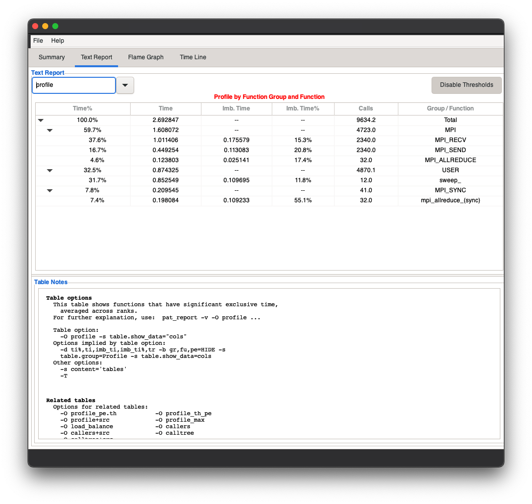
The application displays available views as selectable tabs:

Summary
Text Report
Flame Graph
Time Line (if timeline information is available)

Apprentice3 is set up as a multi-document application and displays three options:

File/Open - Displays an experiment Chooser screen that opens another experiment window. You can open multiple experiments simultaneously.
File/Close - Closes the current experiment window.
Help - Provides limited help information.

Working with the Summary screen

The Summary tab shows the:

Experiment Details panel - Provides basic information about the system on which the experiment was run and the parameters used to run it.
Observations panel - Contains a top-level analysis of the experiment results, including identifying potential bottlenecks, possible fixes, and pointers where to look further.

You can drag the divider between the two panels to change its size.

Working with the Report View screen

The Text Report tab accesses the host performance tables:

Report View screen - Text Report tab

The Text Report tab includes the:

Report pull-down menu - Lists 100+ reports, broken into themes. Depending on the settings while running an experiment, not every report is available. A dialog box indicating that no data was gathered during the experiment might appear. This pull-down menu also shows a table related to the currently displayed one.
Report table - Allows you to manipulate the table format. For example, you can widen or shrink the table size, reorder columns, and collapse or expand tree elements.
Disable/Enable Thresholds button - Toggles whether the table can filter smaller entries.
Table Notes section - Displays a detailed explanation of what is contained in the table.

The panel divider can be dragged to grow or shrink the Table Notes section.

Working with the Flame Graph screen

The Flame Graph tab allows you to visualize the time usage of the program aggregated into each distinct call stack:

Flame Graph tab

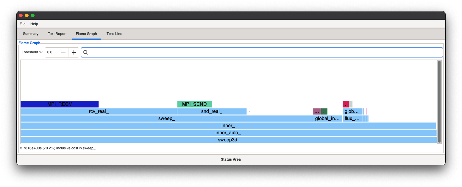
The Flame Graph tab shows each function in a box that is scaled to the time spent in that function. Afterwards, every function it calls upon is put into a proportionally sized box above it.

In the above example, nearly the entire run time is spent in the inner_ call, and much of the time in inner_ is spent in calls to sweep_, global_int_sum_, flux_err_ and several lesser contributors. Retrieve full name and more detailed information by hovering over the box.

The time spent exclusively inside the inner_ function is indicated by the amount of the box with nothing above it.

Clicking a box recenters the display on that function. Clicking global_in.. updates the flame graph:

Flame Graph Focus tab

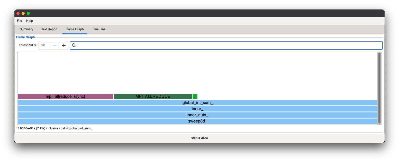
From the Flame Graph Focus tab, you can widen the focus again by clicking a box below the current focus.

The functions in the display are color-coded. MPI function or synchronizing calls are displayed in different colors.

Working with the Time Line screen

Working with Panels

Information shown under the Time Line tab allows you to relate GPU activity against your running program for every thread. You can also zoom in on the activity at any time in the run.

Time Line tab

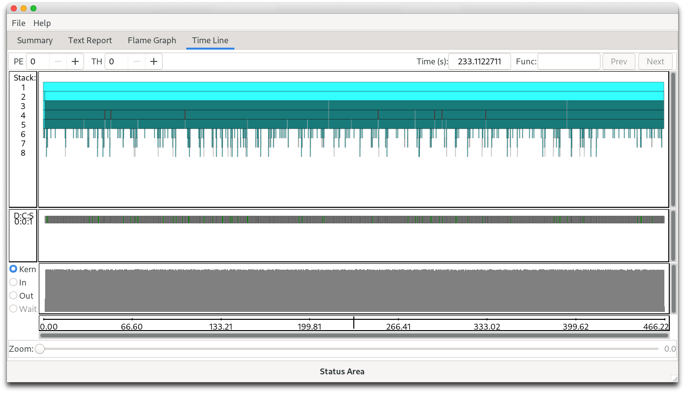
Screen sections shown include the:

Navigation bar
- PE selects the “program element”, the CPU process to display.
- TH selects the CPU thread on the current PE.
- Time shows the time of the center of the display range. You can edit this to recenter to a new interval.
- Func/Prev/Next lets you navigate between occurrences of a specific function.
Stack section

This screen section shows the graphical view of your program stack. Each box shows the beginning and end of a CPU function call. Hover over a box to view the details: function name, call start and end times.
D:C:S (Device/Context/Stream)

The section (to the left) on this row (where D:C:S appears) details the coordinates of the GPU threads associated with the current threads. This information is listed as indexes of the Device (D), Context (C), and Stream (S). Context and Stream are generalized terms since GPU manufacturers use their own nomenclatures.

The section (to the right) on this row is a color-coded bar indicating the processing type:
- Gray: Computation
- Green: Communication
- Empty: Idle
Clicking a rectangle in this display highlights its corresponding CPU call which can be earlier in the timeline due to device lag.
GPU activity

GPU activity includes a graph of the amount of GPU activity at each time. You can select:
- Kernel compute activity
- In data flow into the GPU
- Out data flow out of the GPU
Navigation bars
- Panning Bar: Moves the display interval at the same resolution. It moves back to the center if you release the mouse to pan farther.
- Zoom: Allows you to narrow or widen the view interval. The scale is logarithmic.

Using the Lasso for intervals

You can drag and drop elements within the GPU activity section to set the focus interval directly:

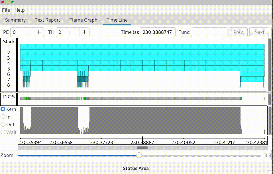
Time Line Navigation tab - Clicking and dragging GPU activity elements

Using the mouse scroll wheel

Use your mouse scroll wheel to zoom in or out on the displayed screen. If you have a two-axis scroll, you can pan with the second axis.

HPE Cray Reveal

Reveal mainly assists users in selecting loops that can be parallelized and then generate the Open MP directive that instructs the compiler to parallelize those loops. Reveal requires a CCE-generated program library that identifies all loops in the application. Select one or more loops for more automated detailed scoping analysis, and then have Reveal generate the Open MP directive. Optionally, Reveal inserts the generated directive in the proper place in the source file.

With only the program library loaded, the tool sorts application loops by file or function. With the addition of performance data loaded into the tool, a list of loops by time and a nested loop view are also available.

Reveal allows the user to modify the scope of one or more variables after the automated scoping analysis is complete. These user changes modify the generated Open MP directive.

A typical way to use Reveal is:

Using CCE, compile the source code to generate a program library.
Generate performance data from a run of the application using the perftools-lite-loops module.
Run Reveal with the program library and attached performance data.
Select loops for scoping analysis.
Scope the loops.
Generate and insert the OpenMP directive(s).
Recompile and test the application.

HPE Cray Reveal dependencies

Reveal only works with CCE, which is provided by the module PrgEnv-cray. Load PrgEnv-cray before running Reveal.
Reveal runs on the login node and requires that X forwarding is enabled. This process allows Reveal windows to be displayed on a laptop or workstation.
A native Mac version of Reveal must be installed. The installer is located in $CRAYPAT_ROOT/share/desktop_installers. Xquartz is required on the Mac for both the native version and the X forwarding mechanism described in number 2.
No Windows or stand-alone Linux installers are provided or supported for Reveal.

Begin using HPE Cray Reveal

Load the perftools-base module:
```
$ module load perftools-base
```
Launch Reveal:

a. Launch Reveal with no parameters:
```
$ reveal
```
If no files are specified on the command line, open an existing program library file by selecting File -> Open.

b. Launch Reveal to open a specific program library file:
```
$ reveal <my_program_library>
```
c. Launch Reveal to open both a program library file and the Perftools-generated runtime performance data files:
```
$ reveal <my_program_library> <my_performance_data_directory>
```
This command launches Reveal and opens both the compiler-generated program library directory and the Perftools-generated runtime performance data files, thereby enabling users to correlate performance data captured during program execution with specific lines and loops in the original source code.

HPE Cray Reveal help

Reveal includes an integrated help system. All other information about using Reveal is presented in the help system, which is accessible whenever HPE Cray Reveal is running by selecting Help from the menu bar.

Generate loop performance data

Loop performance data is generated by compiling and linking an application using a CCE compiler with the perftools-lite-loops module loaded and then running the resulting executable. Follow these steps:

Load the necessary modules:

$ module load PrgEnv-cray
$ module load perftools-base
$ module load perftools-lite-loops

Compile, link, and run the program as usual. The loop performance data directory is created in the current working directory.

Generate a program library

Follow these steps to generate a my_program_library file:

Load the necessary modules. Note that the perftools-lite-loops module should not be loaded when building a program library:
```
$ module load PrgEnv-cray
$ module unload perftools-lite-loops
```
Compile the program using a CCE compiler with the option to build a program library:
- For Fortran, use -h pl=<my_program_library>
- For C/C++, use -f cray-programming-library-path=<my_program_library>
This action generates <my_program_library> in the current working directory.

Note that the program library must be kept with the program source. Moving just the my_program_library file to another location and then opening it with Reveal is not supported.

Compatibilities, Incompatibilities, and Differences

None.

CPE Performance Analysis Tools User Guide

About the HPE Performance Analysis Tools user guide

HPE Performance Analysis Tools

Overview of HPE Cray Apprentice2

Source code analysis using Reveal

Available help

HPE Cray Perftools help

HPE Cray Apprentice2 help

HPE Cray Reveal help

Reference files

HPE Cray Perftools

Instrument the Program

Automatic Profiling Analysis Introduction

MPI Automatic Rank Order Analysis Introduction

pat_opts

Instrumenting a program using pat_run

Run the Program and Collect Data

Analyze the Results

Initial Analysis Using pat_report

HPE Cray Perftools-lite

Instrumentation module options

Getting started with HPE Cray Perftools-lite

Generated output

Disable HPE Cray Perftools-lite

Use HPE Cray Perftools-lite

Use pat_build

Program instrumentation

Basic profiling

Use automatic profiling analysis

Use Predefined Trace Groups

Trace User defined Functions

Enable Tracing and the CrayPat API

Instrument a Single Function

Prevent Instrumentation of a Function

Instrument a User defined List of Functions

Create New Trace Intercept Routines for User-defined Functions

CrayPat API for Advanced Users

Use CrayPat API Calls

Header Files

CRAYPAT Macro

API Calls

Using pat_run

HPE Cray CrayPat runtime environment

Control runtime summarization

Select a predefined experiment

Trace-enhanced sampling

Improve tracebacks

Measure MPI load imbalance

Monitor performance counters

Hardware counters

Accelerator counters

Power management counters

Use pat_report

Generate text reports

Experiment data directories and files

Generate Reports

Predefined Reports

User-defined Reports

Export Data

pat_report Environment Variables

Automatic Profiling Analysis

MPI Automatic Rank Order Analysis

Use Automatic Rank Order Analysis

Force Rank Order Analysis

-O mpi_sm_rank_order

-O mpi_rank_order

-O mpi_hy_rank_order

Observations and Suggestions

Use HPE Cray Apprentice2

Launch Apprentice2

Open Data Files

Basic Navigation

View Panels

Overview Report

Profile Report

Text Report

Traffic Report

Mosaic Report

Activity Report

Call Tree

`pat_opts`

Using pat_run 

User-defined Reports 

`pat_report` Environment Variables

`-O mpi_sm_rank_order`

`-O mpi_rank_order`

`-O mpi_hy_rank_order`